 Back
to HATs
 Back
to HATs Back
to HATs |
A general, and generally accepted definition of a community is: "any assemblage of populations of living organisms in a prescribed area or habitat". This is the definition used by Krebs (1978) who also provides further consideration of various aspects of community ecology. There is a theoretical concept of a community as a group of species which are likely to occur together; in botanical terms, this would be an "association", an idealized community, whilst a "stand" is an actual group of co-occurring plant species as observed in the field. These different concepts are clearly used by plant ecologists and may also be applied to animal communities.
There are many different approaches to the study of a community. The functional inter-relationships between the species (in terms of energy flow, food webs, predator-prey interactions, etc.) are influential in maintaining the integrity of a community and thus worth investigating. Of central importance, though, is the structure of the community in terms of the species which compose it; this determines the functional processes within the community at the same time as being the result of them.
A pragmatic approach is to obtain information encompassing the full
range of species and reflecting their relative abundances. The assumption
then is that the abundance of a species is a reflection of its importance
in the community. Such a representation could be termed a biocoenosis as
in some European work. A subset of the entire assemblage is termed a taxocene
and is so described if interest is restricted to a particular taxonomic
group such as spiders, beetles, etc. Such an approach is commonly adopted,
often for practical reasons, and justified by a degree of ecological uniformity
within the selected taxon. Thus the ecologist can work within these self-imposed
limits and obtain information on species composition. From the data a variety
of descriptive parameters can be calculated for the sample and by implication,
for the community (population) from which the sample is drawn.
Whether a community has many individuals and/or many species is only a partial description of its structure. The number of individuals in each of the differcnt species is an important aspect and species diversity indices make use of this. Consider a community A dominated by a certain species; additional samples probably will merely add more individuals of this species to the collection. Contrast this with a community B in which the constituent species are evenly abundant; in this case additional captures are more likely to belong to new species. Community B could be considered more diverse than community A. Thus a significant feature of species diversity is that it depends not only upon the number of species (richness) but also upon the distribution of individuals between species, i.e. the number of individuals in each species (evenness). More detailed treatments of species diversity are given, for example, by Uetz (1974), Hurlbert (1971), Krebs (1978, ch. 23) and Pianka (1978, pp 286-299).
Indices of species diversity may be based on (a) the actual numbers of individuals in each species, or (b) their relative numbers (proportions of total). The former often depends on the recognition that usually in a community there are many species each represented by a few individuals, and progressively fewer species represented by larger numbers of individuals. A plot of the number of species, S(n), represented by n individuals against n forms a hollow curve considered to approximate to a logarithmic series in which the relationship between the total number of species, S, and total number of individuals, N, is given by S = α loge (1 + N/α ), The constant, α , is Fisher's index of diversity (Krebs (1978), p. 450). Other geometric scales (logarithmic to different bases) may be used in plotting the species abundance curve, e.g. the octave scale (log2). A thorough consideration is given by May (1975).
Examples of diversity indices based on the proportional representation of species: pi = ni/N, ni being number of individuals of species i, include an index of dominance, D, calculated as the sum of the squared proportions for all species; in mathematical notation D = Σ pi2 , for i=1 to S. The reciprocal of this, B = 1 / Σ pi2, for i=1 to S, is an effective index of diversity with a minimum value tending to unity (only one species present or very dominant) and a maximum equal to the number of species (when they are present in equal proportions). Also based on pi is the commonly-used, but in biological terms not particularly informative, Shannon index of diversity, H = - Σ pi· log(pi), for i=1 to S. The base of the logarithms used is commonly 2, although natural logs (to the base e) or log10 are often used. The range of this index is from zero to log S. H is intended to suit the case where the collection is treated as a random sample from the (statistical) population; it reflects the uncertainty of identity of a random individual.
Hurlbert (1971) considers the various indices and proposes one intended to be biologically meaningful. This is the probability of interspecific encounter, PIE = (N/(N - 1))·(1 - Σ pi2), for i=1 to S, intended to reflect the possible degree of interactions between the species in the community. This has a maximum value of unity for an absurdly simple community of two species, each with one individual. For a real community, the more evenly represented the species the closer PIE is to unity.
For all of these indices based on pi, the evenness component of species diversity may be calculated as the ratio of the observed value to the maximum possible value for the observed number of species (except for D).
The evaluation of such descriptive parameters permits objective comparison of communities. Other indices may be used for explicit comparison of communities, again based on either (a) actual numbers of individuals, or (b) relative proportions. An example in category (a) would be a simple Euclidean distance measure, Ejk = √ Σi=1 to S (nij - nik)2, in which nij and nik are the number of individuals of species i in communities j and k respectively. (Believe it or not, this merely amounts to the application of Pythagoras' theorem in a multidimensional hyperspace!) The overlap index, C, is an example of category (b) calculated as Cjk = 1 - ½ pij - pik , in which pij and pik are the proportional representation of species i in communities j and k respectively and the expression pij - pik means that the sign of the difference is ignored.
Any tendency for a sampling method to distort the relative capture rates
for the species will have consequent effects on values obtained for these
descriptive parameters.
Much ecological work is centred on the simplification of complex
data and the parameters considered above are a contribution to this. Superficially,
it would seem that the simplest parameters to evaluate (and quote) are
S, the number of species and N, the number of individuals, in a sample
collected from the community in a standard fashion. For better or worse,
depending on your point of view, different sampling methods vary the capture
rate for different species and thus affect the values of S and N. One could
thus select a sampling method to maximise either S or N, but in doing so
might obtain misleading values for the other, more informative, community
parameters; the problem then is to decide which, if any, of the values
most accurately reflect the true community.
The hypothetical data shown in Table I illustrate this, considering
three collections of 1000 specimens from contrasting sampling methods applied
to a community of 100 species. Method 1 may be taken to give the most accurate
image of the community, dominated by one species with 500 specimens but
with many rare species. Method 2 is biased towards this dominant species,
but against the rarer ones; for unit effort this method would yield highest
values of N, but for the standard sample size of 1000 individuals it includes
much fewer species. In marked contrast, the efficiency of method 3 is inversely
proportional to the abundance of a species so that in the 1000-specimen
sample each of the 100 species is represented by 10 individuals. The resulting
values for some community parameters are indicated in Table I, and the
community structure illustrated in Fig. 1(a, b, c).
TABLE I. Hypothetical data from three contrasting sampling methods (see
text) and corresponding community parameters.
S (n) no. of species represented by n individuals |
|||
| Method: | 1 | 2 | 3 |
| n:
(no. of individuals in species) |
|||
| 1 | 44 | 6 | 0 |
| 2 | 20 | 5 | 0 |
| 4 | 10 | 5 | 0 |
| 8 | 5 | 1 | 0 |
| 10 | 0 | 0 | 100 |
| 16 | 3 | 2 | 0 |
| 32 | 1 | 1 | 0 |
| 64 | 2 | 1 | 0 |
| 128 | 1 | 1 | 0 |
| 500 | 1 | 0 | 0 |
| 700 | 0 | 1 | 0 |
| S - number of species: | 87 | 23 | 100 |
| N - number of specimens: | 1000 | 1000 | 1000 |
| Index of dominance, D: | 0.277 | 0.512 | 0.010 |
| Index of diversity, B: | 3.610 | 1.952 | 100.000 |
| Index of diversity, H: | 2.237 | 1.184 | 4.605 |
| Index of diversity, PIE: | 0.724 | 0.488 | 0.990 |
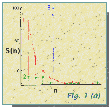
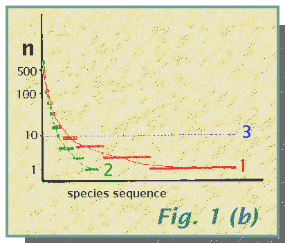
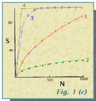
The community structure, shown as a species frequency diagram in Fig. la and species importance curves in Fig. lb, influences the number of species recorded for a given sample size. This is shown in Fig. lc in which the expected values of S for N = 100, 200, 300... are shown. (This calculation of the expected number of species for a standard value of N may be used as a useful indicator of species diversity). These expected values of S have been calculated using the method of Heck, van Belle and Simberloff (1975). The differing rates of species accumulation with increasing N are obvious. They may be compared with that for a rather peculiar sampling procedure which selects for species so that each animal captured is of a different species from the previous one. This method 4 produces a steep, straight line with the capture of all 100 species in the first 100 individuals, and thereafter a straight line of zero slope. Note that the curve for method 3 comes closest to this and is the only one which, in the 1000 specimens, records all 100 species.

(a) Species frequency diagram.
S(n), the number of species represented by n individuals, is plotted
against n on an octave (log2) scale, i.e. 1, 2, 4, 8, 16, 32,
64 and 128, with the dominant species for method
1 (red, open circles) at 500 and for method
2 (green, solid symbols) at 700 individuals. The three methods contrast
with each other, especially method 3 (blue,
triangle) with all 100 species having 10 individuals each.

(b) Species importance curves
show the number of individuals, n, in each species, plotted approximately
against a log2 scale. The species are arranged (from left to
right) in a sequence from most to least abundant. Individual points are
not drawn for method 3 in which each of the
100 species has 10 individuals; the dotted straight line represents this.
The curves for methods 1 and 2
show different slopes, method 1 having many
more rare species than method 2.

(c) Plot of S, total number of species, against N, total number of
individuals
for methods 1, 2,
3
and 4. The points for methods 1,
2,
and 3 are the "observed" values for 1000 individuals
and "expected" values for smaller samples. The different species richness
which would be apparent for the same sample size of the three methods is
clear. Note the proximity of the curve for method
3 to that for the species-selective
method
4 (see text).
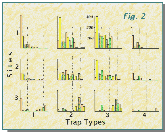
Pitfall traps of different efficiency have been assessed in sampling for spiders in woodland and moorland habitats. In the woodland study at three sites in the Loch Lomond National Nature Reserve, four types of pit-traps, based on plastic jars 6cm diameter by 8cm deep with drainage holes 1.5cm below rim were used: 1. control, plain jars; 2. detergent, 1-2% teepol solution 1-2cm deep in trap; 3. trapping fluid, as 2 incorporating 4% formalin; 4. dry, as 1 but with a horizontal, opaque cover to exclude rainwater (and litter). These were placed at each site in a particular arrangement to account for environmental variations. Analysis of variance indicated differences in efficiency in terms of numbers of individuals and of species captured. Examination of data for the full year starting October 1976 showed significant effects in terms of community parameters, considered more fully by Curtis (1980). Based on the year's catch of 130 species, 11032 individuals, Fig. 2 illustrates the varying capture rates for the more abundant species (data in Table 1 of Curtis, 1980).
Fig. 2. Histograms showing the numbers of individuals in the
17 more abundant species of harvestmen and spiders captured in four types
of pit-trap at three woodland sites. 
The colouring of the bars and the dotted lines passing through species
5, 10 and 15 are intended to facilitate comparison. Note the contrasting
shapes of the histograms and the differences for single species, especially
species 1, with peak of 306 in type 1 traps at site 1 (converse of most
other species), species 2, with more marked differences between trap-types
at site 2, and species 4 which at site 1 is captured most in type 3 traps,
but most in type 2 traps at sites 2 and 3. The species, 1 to 17, are:-
Opiliones: Nemastoma bimaculatum, Oligolophus tridens, Lacinius
ephippiatus.
Araneida: Macrargus rufus, Lepthyphantes zimmermanni, L. tenebricola,
Dicymbium tibiale, Monocephalus fuscipes, Diplocephalus latifrons, D. picinus,
Centromerus sylvaticus, Tapinocyba pallens, Cnephalocotes obscurus, Pirata
hygrophilus, Alopecosa pulverulenta, Trochosa spinipalpis, Pardosa amentata.
(Data from Curtis, 1980, Table 1).
The influence of trap efficiency is clear in the different shapes of the histograms. There are consequently significant effects on the community parameter values derived from the samples because the variations in trap efficiency are not the same for the various species, nor for different habitats and seasons. A particular feature is that the expected number of species for a given sample size (taken for 100 adults) is markedly dependent on trap-type.
The moorland study of Curtis (1979) compared formalin/teepol pit-traps
with pitfalls containing saturated picric acid. Again, different relationships
between S and N were evident and reflected in variations in community parameter
values. Table II indicates the values obtained for diversity indices at
three sampling stations in Glen Finart, Argyll. Although based on rather
smaller samples, the community parameters clearly differ between trap-types,
the distortion varying from one station to another.
TABLE II. Data of Curtis (1979), from two types of pitfall trap, FT
with formalin/teepol and PA with saturated picric acid; N = no of individuals
captured, S = no. of species, diversity is expressed in terms of the indices
B, H, PIE and the number of species expected in a sample of 20 adults,
E(S) (± standard deviation).
| Sample station in Glen Finart | Trap Type | N | S | E(S) | B | H | PIE |
| A | FT
PA |
43
47 |
12
10 |
8.4 ± 1.2
6.9 ± 1.1 |
6.02
3.60 |
2.06
1.69 |
0.86
0.74 |
| B | FT
PA |
73
23 |
21
10 |
12.4 ± 1.5
9.7 ± 0.5 |
13.13
8.34 |
2.79
2.20 |
0.94
0.92 |
| C | FT
PA |
141
74 |
6
7 |
2.3 ± 0.9
2.9 ± 1.1 |
1.16
1.22 |
0.36
0.48 |
0.14
0.18 |
So one can select the sampling method which seems most appropriate or most efficient. Then, as long as one applies the same method to each of the communities under consideration it is feasible to make valid comparisons - or is it? The data distortions and problems of interpretation explicitly described for pitfall trapping will apply to any sampling method (Curtis, 1980). The distortions are habitat-dependent, so problems ensue if the communities are in different habitats.
The data distortions depend directly on the responses of the various
species to the sampling methnd, so one might argue that unless the species
compositions of the communities are identical the distortions will differ
between them and, if one is very pessimistic, thereby invalidate any comparison.
However, it could be said that as long as between-community variations
in efficiency only apply to species which are absent from one of the communities
then one can conclude that they differ in spccies composition but must
realise that precise description of the difference is dependent on the
particular species. The curvilinear relationship between S and N, i.e.
that if your sample size is large enough you will record most species,
may be used to ease one's mind. However, this only applies if one is considering
just species richness; interpretive problems still remain if one is interested
in other, potentially more informative, community parameters.
I am grateful for the continued support of Prof. J. C. Smyth, for
sampling assistance from Mr H. G. Stewart, for long-term co-operation from
the Nature Conservancy Council. and for valuable discussions with many
students and colleagues, especially Dr E. Bignal.
CURTIS, D. J., 1980. Pitfalls in spider community studies (Arachnida, Araneae). J. Arachnol., 8: 271-280.
DUFFEY, E., 1972. Ecological survey and the arachnologist. Bull. Brit. Arach. Soc., 2: 69-82.
DUFFEY, E., 1974. Comparative sampling methods for grassland spiders. Bull. Brit. Arach. Soc., 3: 34-37.
HECK, Jr., K. L., C. VAN BELLE & D. SIMBERLOFF, 1975. Explicit calculation of the rarefaction diversity measurement and the determination of sufficient sample size. Ecology, 56: 1459-1461.
HURLBERT, S. H. 1971. The non-concept of species diversity; a critique and alternative parameters. Ecology, 52: 577-586.
KREBS, C. J. 1978. Ecology. 2nd ed. Harper & Row, New York.
MAY, R. H., 1975. Patterns of species abundance and diversity, pp. 81-120 in Cody, M. L. & J. M. Diamond (eds) Ecology and evolution of communities. Bellknap Press of Harvard University Press, Cambridge, USA.
PIANKA, E. R., 1978. Evolutionary ecology. 2nd ed. Harper & Row, New York,
SOUTHWOOD, T. R. E. 1966. Ecological methods. Chapman & Hall, London,
UETZ, C. W., 1974. Species diversity: a review. Biologist, 56: 111-129.
UETZ, C. W., & J. M. Biere, 1980. Prey of Micrathena gracilis
(Walckenaer) (Araneae: Araneidae) in comparison with artificial webs and
other trapping devices. Bull. Brit. Arach. Soc., 5: 101-107.
| Return to..? |  Back
to HATs Back
to HATs |
|
 Ariadne Home Page
 |
||