Back to HATs
 
 

Ordination

This means "putting into order" F arranging data points in sequence relative to a continuous axis or axes.

e.g. If you have a series of samples with the abundances of just one species, you can place them in order of increasing (or decreasing) abundance along a single axis - here we have 26 samples (A - Z).
 

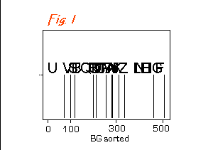
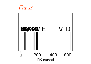Their positions depend on the abundance of species 'BG' (actually Black-headed Gull Larus ridibundus) in Fig. 1
 
 

and species 'RK' (which is Redshank Tringa totanus) in Fig. 2
.
 
 
 

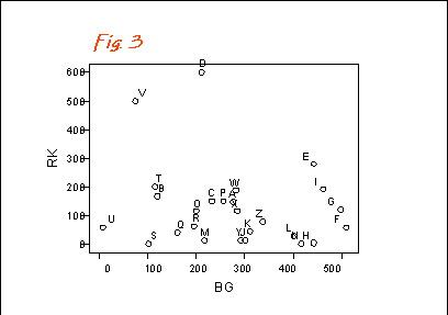
Or if you have two species, you can plot one against the other, as with the two species of birds:-

Here once again, RK is redshank and BG is Black-headed Gull.
 
 
 
 
 

BUT - what do you do if you have more than two species.

If, to our data on a gull and a wader, we now include data on a second wader - the Dunlin Calidris alpina (DN).

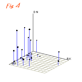At a pinch, you can do three-dimensional plots as in Fig. 4, where we have BG and RK on the x and y axes and DN plotted on the z axis, with all three axes being orthogonal to each other.

We could use even  more complicated respresentations,
but the optimal solution is to apply an ordination algorithm so that we derive compound axes based on all the species and use the best two of these axes to generate a straightforward two-dimensional plot..
 
 
 
 
 

There are many ordination algorithms used in ecology; four "popular" ones are listed here:

PCA Principal Components Analysis

WA Weighted Averages

RA Reciprocal Averaging = CA Correspondence Analysis

DCA De-trended Correspondence Analysis.
 
 

All of these share the aim of generating axes based upon some combination of the original variables, such that if two of these are plotted against each other they (a) show as much as possible of the variation in the data and (b) minimise any distortion interms of the relative positions of the data points.
 

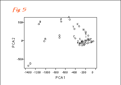
Thus all seven bird species for the 26 data points in our little data-set can be used with PCA to generate principal axes. The result is shown in Fig. 5.

In this case, when the first of these PCA axes is plotted against the second, the resultant graph expresses about 90% of the overall variation and the relative positions of the different samples are readily seen.

Each of these axes represents a combination of the original birds, the "principal score" for each sample is calculated as a weighted sum of the original variables (the abundances of the individual bird species).
 
 
 
 
 
 
 

The relative contributions of the different species can also be plotted, as shown in Fig. 5.  The positions of the species in this plot reflect their relative occurrence in the different samples. In this way, any species groupings are revealed.

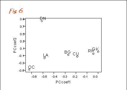
BG Black-headed Gull

CU Curlew

DN Dunlin

GK Greenshank

LA Lapwing

OC Oystercatcher

RK Redshank
 
 
 

As well as showing the weightings of these birds' contributions to the principal component scores, their relative positions also give an indications of the species' similarities or differences in terms of their distributions between the samples.

Thus , the ordination approach gives information both about the samples and the variables which are used.